TensorFlow

Edited March 1, 2022 by Suresh Kumar Balasundaramsivaprakash and Pankaj Dange

Introduction

TensorFlow is an end-to-end open-source platform for machine learning. It has a comprehensive, flexible ecosystem of tools, libraries, and community resources that lets researchers push the state-of-the-art in ML and developers easily build and deploy ML powered applications.

This notebook provides a basic starting point and boilerplate code for Tensorflow 2.0 with respect to Model creation and training.

The approach followed is to create, train, evaluate Models with the same architecture, same MNIST dataset using different ways of building Models from basic to the advanced method and different ways of training at a basic level.

Import Libraries

Below are some basic Libraries related to Tensorflow and Keras

import tensorflow as tf
from tensorflow import keras
from tensorflow.keras import Model
from tensorflow.keras.layers import Input,Layer,Dense,Flatten

Below are Libraries for needed to manupulate and visualize

import numpy as np
import pandas as pd
import matplotlib.pyplot as plt

MNIST dataset

The MNIST dataset has handwritten digits as image files. It has a training set of 60,000 examples, and a test set of 10,000 examples

Import MNIST dataset

Different ways of Building Model

Keras datasets library has the mnist dataset inbuilt

mnist = tf.keras.datasets.mnist

(x_train,y_train),(x_test,y_test)=mnist.load_data()

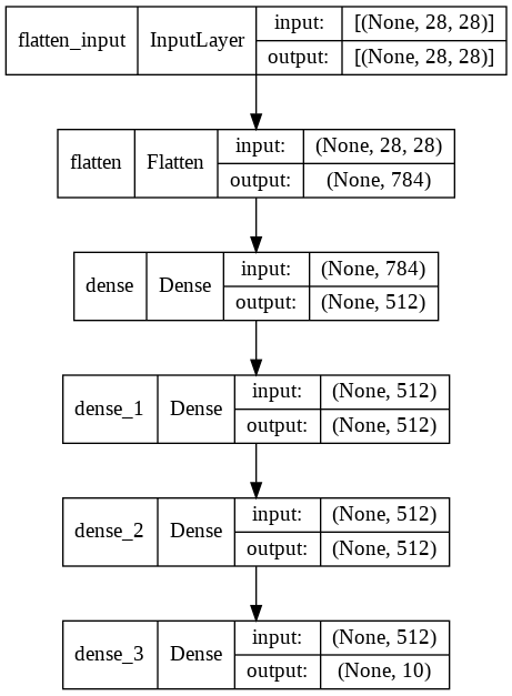
Sequential Model

A Sequential model is appropriate for a plain stack of layers where each layer has exactly one input tensor and one output tensor.

Model Architecture

def create_model():
  model=tf.keras.models.Sequential([
  tf.keras.layers.Flatten(input_shape=(28,28)),
  Dense(units=512,activation=tf.nn.relu),
  Dense(units=512,activation=tf.nn.relu),
  Dense(units=512,activation=tf.nn.relu),
  Dense(units=10,activation=tf.nn.softmax)])
  return model

Create Model

model=create_model()

Model Summary

model.summary()

Model: "sequential"
_________________________________________________________________
 Layer (type)                Output Shape              Param #   
=================================================================
 flatten (Flatten)           (None, 784)               0         
                                                                 
 dense (Dense)               (None, 512)               401920    
                                                                 
 dense_1 (Dense)             (None, 512)               262656    
                                                                 
 dense_2 (Dense)             (None, 512)               262656    
                                                                 
 dense_3 (Dense)             (None, 10)                5130      
                                                                 
=================================================================
Total params: 932,362
Trainable params: 932,362
Non-trainable params: 0
_________________________________________________________________

Visualize Model

keras.utils.plot_model(model, show_shapes=True)

png

Compile Model

Compile step is a key step that users Optimizer, Loss fuction and Metrics used for Back propagation. Please refer below high level insignt

The Loss Function is one of the important components of Neural Networks. Loss is nothing but a prediction error of Neural Net. And the method to calculate the loss is called Loss Function. In simple words, the Loss is used to calculate the gradients. And gradients are used to update the weights of the Neural Net.

Optimizers are algorithms or methods used to change the attributes of your neural network such as weights and learning rate in order to reduce the losses. Optimizers help to get results faster.

Metrics can be accuracy, loss etc to assess the performance of Trained model

model.compile(optimizer=tf.keras.optimizers.Adam(learning_rate=0.001), metrics=['accuracy'],loss='sparse_categorical_crossentropy')

Train Model

Trains the model for a fixed number of epochs. At each epoch the weights are adjusted through back probagation.

We can see every epoc the sparse_categorical_crossentropy loss is reduced and the train accuracy is increased

model.fit(x_train,y_train,epochs=15,batch_size=1024)

Epoch 1/15
59/59 [==============================] - 1s 3ms/step - loss: 8.4750 - accuracy: 0.7977
Epoch 2/15
59/59 [==============================] - 0s 3ms/step - loss: 0.3311 - accuracy: 0.9366
Epoch 3/15
59/59 [==============================] - 0s 3ms/step - loss: 0.1572 - accuracy: 0.9632
Epoch 4/15
59/59 [==============================] - 0s 3ms/step - loss: 0.0824 - accuracy: 0.9789
Epoch 5/15
59/59 [==============================] - 0s 3ms/step - loss: 0.0419 - accuracy: 0.9883
Epoch 6/15
59/59 [==============================] - 0s 3ms/step - loss: 0.0206 - accuracy: 0.9950
Epoch 7/15
59/59 [==============================] - 0s 3ms/step - loss: 0.0103 - accuracy: 0.9980
Epoch 8/15
59/59 [==============================] - 0s 3ms/step - loss: 0.0052 - accuracy: 0.9996
Epoch 9/15
59/59 [==============================] - 0s 3ms/step - loss: 0.0030 - accuracy: 0.9999
Epoch 10/15
59/59 [==============================] - 0s 3ms/step - loss: 0.0021 - accuracy: 0.9999
Epoch 11/15
59/59 [==============================] - 0s 3ms/step - loss: 0.0016 - accuracy: 1.0000
Epoch 12/15
59/59 [==============================] - 0s 3ms/step - loss: 0.0013 - accuracy: 1.0000
Epoch 13/15
59/59 [==============================] - 0s 3ms/step - loss: 0.0011 - accuracy: 1.0000
Epoch 14/15
59/59 [==============================] - 0s 3ms/step - loss: 9.3821e-04 - accuracy: 1.0000
Epoch 15/15
59/59 [==============================] - 0s 3ms/step - loss: 8.2369e-04 - accuracy: 1.0000





<keras.callbacks.History at 0x7f89e01bcc50>

Evaluate Model with Test data

Test data is used evaluate the performance of the model trained.

testaccuracy=model.evaluate(x_test,y_test)
print("The test accuracy is :", np.round(testaccuracy[1]*100,2),"%")

313/313 [==============================] - 1s 2ms/step - loss: 0.2533 - accuracy: 0.9586
The test accuracy is : 95.86 %

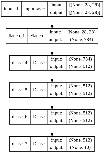
Model built with Functional APIs

The Keras functional API is a way to create models that are more flexible than the tf.keras.Sequential API. The functional API can handle models with non-linear topology, shared layers, and even multiple inputs or outputs.

Model Architecture

def build_model_with_functional():
    
    # instantiate the input Tensor
    input_layer = tf.keras.Input(shape=(28, 28))
    
    # stack the layers using the syntax: new_layer()(previous_layer)
    flatten_layer = tf.keras.layers.Flatten()(input_layer)
    first_dense = tf.keras.layers.Dense(512, activation=tf.nn.relu)(flatten_layer)
    second_dense = tf.keras.layers.Dense(512, activation=tf.nn.relu)(first_dense)
    third_dense = tf.keras.layers.Dense(512, activation=tf.nn.relu)(second_dense)
    output_layer = tf.keras.layers.Dense(10, activation=tf.nn.softmax)(third_dense)
    
    # declare inputs and outputs
    func_model = Model(inputs=input_layer, outputs=output_layer)
    
    return func_model

Create, Visualize, Train and evaluate the model

The same steps explained in sequential model is consolidated here as they are exactly same code

model=build_model_with_functional()
model.compile(optimizer=tf.keras.optimizers.Adam(learning_rate=0.001), metrics=['accuracy'],loss='sparse_categorical_crossentropy')
model.fit(x_train,y_train,epochs=5,batch_size=1024)
testaccuracy=model.evaluate(x_test,y_test)
print("The test accuracy is :", np.round(testaccuracy[1]*100,2),"%")

Epoch 1/5
59/59 [==============================] - 1s 3ms/step - loss: 9.2116 - accuracy: 0.7801
Epoch 2/5
59/59 [==============================] - 0s 3ms/step - loss: 0.3370 - accuracy: 0.9315
Epoch 3/5
59/59 [==============================] - 0s 3ms/step - loss: 0.1733 - accuracy: 0.9567
Epoch 4/5
59/59 [==============================] - 0s 3ms/step - loss: 0.0960 - accuracy: 0.9736
Epoch 5/5
59/59 [==============================] - 0s 3ms/step - loss: 0.0526 - accuracy: 0.9858
313/313 [==============================] - 1s 2ms/step - loss: 0.2185 - accuracy: 0.9515
The test accuracy is : 95.15 %

model.summary()

Model: "model"
_________________________________________________________________
 Layer (type)                Output Shape              Param #   
=================================================================
 input_1 (InputLayer)        [(None, 28, 28)]          0         
                                                                 
 flatten_1 (Flatten)         (None, 784)               0         
                                                                 
 dense_4 (Dense)             (None, 512)               401920    
                                                                 
 dense_5 (Dense)             (None, 512)               262656    
                                                                 
 dense_6 (Dense)             (None, 512)               262656    
                                                                 
 dense_7 (Dense)             (None, 10)                5130      
                                                                 
=================================================================
Total params: 932,362
Trainable params: 932,362
Non-trainable params: 0
_________________________________________________________________

keras.utils.plot_model(model, show_shapes=True)

png

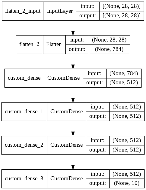
Advanced Model Building Methods

This will be used for some advanced needs. Below are few of them.

To build models with multiple inputs and a single output and vice versa.
To share weights between layers in a model
Custom Computations within layers
Custom gradient function to be used in back probagation

This section shows custom layer method alone. There are other types like custom Methods, custom gradients etc

Custom Layer definition

Custom class is defined using the super class Layer class that we imported. Activation functions, weights are intialized in the build method call funtion does the back probagation and updates the weights of the network

class CustomDense(Layer):

    # add an activation parameter
    def __init__(self, units=32, activation=None):
        super(CustomDense, self).__init__()
        self.units = units
        
        # define the activation to get from the built-in activation layers in Keras
        self.activation = tf.keras.activations.get(activation)


    def build(self, input_shape):
        w_init = tf.random_normal_initializer()
        self.w = tf.Variable(name="kernel",
            initial_value=w_init(shape=(input_shape[-1], self.units),
                                 dtype='float32'),
            trainable=True)
        b_init = tf.zeros_initializer()
        self.b = tf.Variable(name="bias",
            initial_value=b_init(shape=(self.units,), dtype='float32'),
            trainable=True)
        super().build(input_shape)


    def call(self, inputs):
        
        # pass the computation to the activation layer
        return self.activation(tf.matmul(inputs, self.w) + self.b)

Model Architecture

def build_model_with_custom_layer():
  model=tf.keras.models.Sequential([
  tf.keras.layers.Flatten(input_shape=(28,28)),
  CustomDense(units=512,activation=tf.nn.relu),
  CustomDense(units=512,activation=tf.nn.relu),
  CustomDense(units=512,activation=tf.nn.relu),
  CustomDense(units=10,activation=tf.nn.softmax)])
  return model

Create, Visualize, Train and evaluate the model

The same steps explained in sequential model is consolidated here as they are exactly same code

model=build_model_with_custom_layer()
model.compile(optimizer=tf.keras.optimizers.Adam(learning_rate=0.001), metrics=['accuracy'],loss='sparse_categorical_crossentropy')
model.fit(x_train,y_train,epochs=5,batch_size=1024)
testaccuracy=model.evaluate(x_test,y_test)
print("The test accuracy is :", np.round(testaccuracy[1]*100,2),"%")

Epoch 1/5
59/59 [==============================] - 1s 3ms/step - loss: 6.9926 - accuracy: 0.8236
Epoch 2/5
59/59 [==============================] - 0s 3ms/step - loss: 0.3592 - accuracy: 0.9421
Epoch 3/5
59/59 [==============================] - 0s 3ms/step - loss: 0.1580 - accuracy: 0.9664
Epoch 4/5
59/59 [==============================] - 0s 3ms/step - loss: 0.0767 - accuracy: 0.9797
Epoch 5/5
59/59 [==============================] - 0s 3ms/step - loss: 0.0332 - accuracy: 0.9909
313/313 [==============================] - 1s 2ms/step - loss: 0.2930 - accuracy: 0.9522
The test accuracy is : 95.22 %

model.summary()

Model: "sequential_1"
_________________________________________________________________
 Layer (type)                Output Shape              Param #   
=================================================================
 flatten_2 (Flatten)         (None, 784)               0         
                                                                 
 custom_dense (CustomDense)  (None, 512)               401920    
                                                                 
 custom_dense_1 (CustomDense  (None, 512)              262656    
 )                                                               
                                                                 
 custom_dense_2 (CustomDense  (None, 512)              262656    
 )                                                               
                                                                 
 custom_dense_3 (CustomDense  (None, 10)               5130      
 )                                                               
                                                                 
=================================================================
Total params: 932,362
Trainable params: 932,362
Non-trainable params: 0
_________________________________________________________________

keras.utils.plot_model(model, show_shapes=True)

png

Different ways of Training Model

Some of the basic methods of tracking metrics for training and validation and to prevent overfitting.

Tracking Training metrics

model=create_model()
model.compile(optimizer=tf.keras.optimizers.Adam(learning_rate=0.001), metrics=['accuracy'],loss='sparse_categorical_crossentropy')
model.fit(x_train,y_train,epochs=5,batch_size=1024)
testaccuracy=model.evaluate(x_test,y_test)
print("The test accuracy is :", np.round(testaccuracy[1]*100,2),"%")

Epoch 1/5
59/59 [==============================] - 1s 3ms/step - loss: 10.1107 - accuracy: 0.7674
Epoch 2/5
59/59 [==============================] - 0s 3ms/step - loss: 0.3363 - accuracy: 0.9260
Epoch 3/5
59/59 [==============================] - 0s 3ms/step - loss: 0.1724 - accuracy: 0.9547
Epoch 4/5
59/59 [==============================] - 0s 3ms/step - loss: 0.0966 - accuracy: 0.9730
Epoch 5/5
59/59 [==============================] - 0s 3ms/step - loss: 0.0556 - accuracy: 0.9842
313/313 [==============================] - 1s 2ms/step - loss: 0.2094 - accuracy: 0.9520
The test accuracy is : 95.2 %

Tracking Training & Validation metrics

Validation split option given below make the training to calculate valition metrics that will be used for early stopping and overfitting.

If we have validation data separately we can provide validaiton_data=[val_Data,val_labels] instead of validation split.

model=create_model()
model.compile(optimizer=tf.keras.optimizers.Adam(learning_rate=0.001), metrics=['accuracy'],loss='sparse_categorical_crossentropy')
model.fit(x_train,y_train,epochs=50,batch_size=1024,validation_split=0.2)

Epoch 1/50
47/47 [==============================] - 1s 6ms/step - loss: 10.0500 - accuracy: 0.7710 - val_loss: 0.5356 - val_accuracy: 0.9170
Epoch 2/50
47/47 [==============================] - 0s 4ms/step - loss: 0.3576 - accuracy: 0.9307 - val_loss: 0.3286 - val_accuracy: 0.9343
Epoch 3/50
47/47 [==============================] - 0s 4ms/step - loss: 0.1703 - accuracy: 0.9579 - val_loss: 0.2686 - val_accuracy: 0.9443
Epoch 4/50
47/47 [==============================] - 0s 3ms/step - loss: 0.0894 - accuracy: 0.9761 - val_loss: 0.2526 - val_accuracy: 0.9456
Epoch 5/50
47/47 [==============================] - 0s 4ms/step - loss: 0.0485 - accuracy: 0.9865 - val_loss: 0.2398 - val_accuracy: 0.9493
Epoch 6/50
47/47 [==============================] - 0s 4ms/step - loss: 0.0244 - accuracy: 0.9941 - val_loss: 0.2354 - val_accuracy: 0.9517
Epoch 7/50
47/47 [==============================] - 0s 4ms/step - loss: 0.0127 - accuracy: 0.9975 - val_loss: 0.2292 - val_accuracy: 0.9555
Epoch 8/50
47/47 [==============================] - 0s 4ms/step - loss: 0.0065 - accuracy: 0.9994 - val_loss: 0.2286 - val_accuracy: 0.9555
Epoch 9/50
47/47 [==============================] - 0s 4ms/step - loss: 0.0037 - accuracy: 0.9999 - val_loss: 0.2287 - val_accuracy: 0.9561
Epoch 10/50
47/47 [==============================] - 0s 4ms/step - loss: 0.0026 - accuracy: 1.0000 - val_loss: 0.2291 - val_accuracy: 0.9568
Epoch 11/50
47/47 [==============================] - 0s 4ms/step - loss: 0.0021 - accuracy: 1.0000 - val_loss: 0.2285 - val_accuracy: 0.9572
Epoch 12/50
47/47 [==============================] - 0s 4ms/step - loss: 0.0017 - accuracy: 1.0000 - val_loss: 0.2282 - val_accuracy: 0.9578
Epoch 13/50
47/47 [==============================] - 0s 4ms/step - loss: 0.0014 - accuracy: 1.0000 - val_loss: 0.2296 - val_accuracy: 0.9582
Epoch 14/50
47/47 [==============================] - 0s 4ms/step - loss: 0.0012 - accuracy: 1.0000 - val_loss: 0.2291 - val_accuracy: 0.9579
Epoch 15/50
47/47 [==============================] - 0s 4ms/step - loss: 0.0011 - accuracy: 1.0000 - val_loss: 0.2295 - val_accuracy: 0.9584
Epoch 16/50
47/47 [==============================] - 0s 4ms/step - loss: 9.4969e-04 - accuracy: 1.0000 - val_loss: 0.2299 - val_accuracy: 0.9586
Epoch 17/50
47/47 [==============================] - 0s 4ms/step - loss: 8.5186e-04 - accuracy: 1.0000 - val_loss: 0.2299 - val_accuracy: 0.9588
Epoch 18/50
47/47 [==============================] - 0s 4ms/step - loss: 7.6219e-04 - accuracy: 1.0000 - val_loss: 0.2306 - val_accuracy: 0.9588
Epoch 19/50
47/47 [==============================] - 0s 4ms/step - loss: 6.8875e-04 - accuracy: 1.0000 - val_loss: 0.2305 - val_accuracy: 0.9591
Epoch 20/50
47/47 [==============================] - 0s 4ms/step - loss: 6.2304e-04 - accuracy: 1.0000 - val_loss: 0.2305 - val_accuracy: 0.9593
Epoch 21/50
47/47 [==============================] - 0s 3ms/step - loss: 5.7018e-04 - accuracy: 1.0000 - val_loss: 0.2307 - val_accuracy: 0.9598
Epoch 22/50
47/47 [==============================] - 0s 4ms/step - loss: 5.2338e-04 - accuracy: 1.0000 - val_loss: 0.2314 - val_accuracy: 0.9600
Epoch 23/50
47/47 [==============================] - 0s 4ms/step - loss: 4.8150e-04 - accuracy: 1.0000 - val_loss: 0.2315 - val_accuracy: 0.9602
Epoch 24/50
47/47 [==============================] - 0s 4ms/step - loss: 4.4403e-04 - accuracy: 1.0000 - val_loss: 0.2320 - val_accuracy: 0.9603
Epoch 25/50
47/47 [==============================] - 0s 4ms/step - loss: 4.1128e-04 - accuracy: 1.0000 - val_loss: 0.2321 - val_accuracy: 0.9603
Epoch 26/50
47/47 [==============================] - 0s 4ms/step - loss: 3.8172e-04 - accuracy: 1.0000 - val_loss: 0.2326 - val_accuracy: 0.9603
Epoch 27/50
47/47 [==============================] - 0s 4ms/step - loss: 3.5563e-04 - accuracy: 1.0000 - val_loss: 0.2328 - val_accuracy: 0.9602
Epoch 28/50
47/47 [==============================] - 0s 4ms/step - loss: 3.3193e-04 - accuracy: 1.0000 - val_loss: 0.2332 - val_accuracy: 0.9606
Epoch 29/50
47/47 [==============================] - 0s 4ms/step - loss: 3.0909e-04 - accuracy: 1.0000 - val_loss: 0.2336 - val_accuracy: 0.9607
Epoch 30/50
47/47 [==============================] - 0s 4ms/step - loss: 2.9048e-04 - accuracy: 1.0000 - val_loss: 0.2337 - val_accuracy: 0.9609
Epoch 31/50
47/47 [==============================] - 0s 4ms/step - loss: 2.7263e-04 - accuracy: 1.0000 - val_loss: 0.2338 - val_accuracy: 0.9607
Epoch 32/50
47/47 [==============================] - 0s 4ms/step - loss: 2.5543e-04 - accuracy: 1.0000 - val_loss: 0.2339 - val_accuracy: 0.9602
Epoch 33/50
47/47 [==============================] - 0s 4ms/step - loss: 2.4074e-04 - accuracy: 1.0000 - val_loss: 0.2346 - val_accuracy: 0.9610
Epoch 34/50
47/47 [==============================] - 0s 4ms/step - loss: 2.2690e-04 - accuracy: 1.0000 - val_loss: 0.2347 - val_accuracy: 0.9612
Epoch 35/50
47/47 [==============================] - 0s 4ms/step - loss: 2.1398e-04 - accuracy: 1.0000 - val_loss: 0.2350 - val_accuracy: 0.9612
Epoch 36/50
47/47 [==============================] - 0s 3ms/step - loss: 2.0227e-04 - accuracy: 1.0000 - val_loss: 0.2355 - val_accuracy: 0.9619
Epoch 37/50
47/47 [==============================] - 0s 4ms/step - loss: 1.9076e-04 - accuracy: 1.0000 - val_loss: 0.2354 - val_accuracy: 0.9613
Epoch 38/50
47/47 [==============================] - 0s 4ms/step - loss: 1.8179e-04 - accuracy: 1.0000 - val_loss: 0.2358 - val_accuracy: 0.9617
Epoch 39/50
47/47 [==============================] - 0s 4ms/step - loss: 1.7166e-04 - accuracy: 1.0000 - val_loss: 0.2361 - val_accuracy: 0.9618
Epoch 40/50
47/47 [==============================] - 0s 4ms/step - loss: 1.6309e-04 - accuracy: 1.0000 - val_loss: 0.2364 - val_accuracy: 0.9617
Epoch 41/50
47/47 [==============================] - 0s 4ms/step - loss: 1.5517e-04 - accuracy: 1.0000 - val_loss: 0.2367 - val_accuracy: 0.9619
Epoch 42/50
47/47 [==============================] - 0s 4ms/step - loss: 1.4714e-04 - accuracy: 1.0000 - val_loss: 0.2369 - val_accuracy: 0.9617
Epoch 43/50
47/47 [==============================] - 0s 4ms/step - loss: 1.4015e-04 - accuracy: 1.0000 - val_loss: 0.2373 - val_accuracy: 0.9617
Epoch 44/50
47/47 [==============================] - 0s 4ms/step - loss: 1.3339e-04 - accuracy: 1.0000 - val_loss: 0.2376 - val_accuracy: 0.9621
Epoch 45/50
47/47 [==============================] - 0s 4ms/step - loss: 1.2716e-04 - accuracy: 1.0000 - val_loss: 0.2376 - val_accuracy: 0.9618
Epoch 46/50
47/47 [==============================] - 0s 3ms/step - loss: 1.2131e-04 - accuracy: 1.0000 - val_loss: 0.2381 - val_accuracy: 0.9619
Epoch 47/50
47/47 [==============================] - 0s 4ms/step - loss: 1.1598e-04 - accuracy: 1.0000 - val_loss: 0.2382 - val_accuracy: 0.9622
Epoch 48/50
47/47 [==============================] - 0s 4ms/step - loss: 1.1079e-04 - accuracy: 1.0000 - val_loss: 0.2386 - val_accuracy: 0.9622
Epoch 49/50
47/47 [==============================] - 0s 4ms/step - loss: 1.0595e-04 - accuracy: 1.0000 - val_loss: 0.2389 - val_accuracy: 0.9623
Epoch 50/50
47/47 [==============================] - 0s 4ms/step - loss: 1.0133e-04 - accuracy: 1.0000 - val_loss: 0.2391 - val_accuracy: 0.9622





<keras.callbacks.History at 0x7f8af3fbecd0>

Ploting Train vs Test loss


plt.figure(figsize=(10,8))
test_accuracy=model.history.history['val_accuracy']
train_accuracy=model.history.history['accuracy']
epochs_range=range(1,len(test_accuracy)+1)
plt.plot(epochs_range, test_accuracy,'b', linewidth=1,label='Test Accuracy')
plt.plot(epochs_range, train_accuracy,'r', linewidth=1,label='Train Accuracy')
plt.xlabel("Epoch")
plt.ylabel(" Validation accuracy")
plt.title("Model's Train vs Test accuracy ")
plt.legend()
plt.grid()
plt.show()

png

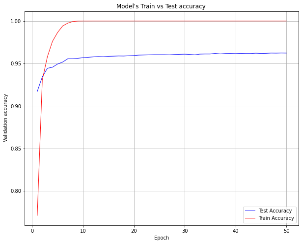
testaccuracy=model.evaluate(x_test,y_test)
print("The test accuracy is :", np.round(testaccuracy[1]*100,2),"%")

313/313 [==============================] - 1s 2ms/step - loss: 0.2527 - accuracy: 0.9617
The test accuracy is : 96.17 %

Early stopping to prevent Overfitting

Below code shows how to do early stopping to prevent overfitting. This code check validation accuracy and if it does not increase for 2 epochs(patience), it stops the train and assigns best possible weights to the model(restore_best_weights=True)

from tensorflow.keras.callbacks import EarlyStopping, ModelCheckpoint
callbacks = [EarlyStopping(monitor='val_accuracy', patience=2,restore_best_weights=True)] # Early Stopping

model=create_model()
model.compile(optimizer=tf.keras.optimizers.Adam(learning_rate=0.001), metrics=['accuracy'],loss='sparse_categorical_crossentropy')
model.fit(x_train,y_train,epochs=50,batch_size=1024,validation_split=0.2,callbacks=callbacks)

Epoch 1/50
47/47 [==============================] - 1s 7ms/step - loss: 10.0079 - accuracy: 0.7644 - val_loss: 0.5353 - val_accuracy: 0.9054
Epoch 2/50
47/47 [==============================] - 0s 4ms/step - loss: 0.3624 - accuracy: 0.9224 - val_loss: 0.3240 - val_accuracy: 0.9300
Epoch 3/50
47/47 [==============================] - 0s 4ms/step - loss: 0.1776 - accuracy: 0.9545 - val_loss: 0.2734 - val_accuracy: 0.9358
Epoch 4/50
47/47 [==============================] - 0s 4ms/step - loss: 0.0989 - accuracy: 0.9733 - val_loss: 0.2493 - val_accuracy: 0.9415
Epoch 5/50
47/47 [==============================] - 0s 4ms/step - loss: 0.0562 - accuracy: 0.9852 - val_loss: 0.2348 - val_accuracy: 0.9466
Epoch 6/50
47/47 [==============================] - 0s 4ms/step - loss: 0.0312 - accuracy: 0.9924 - val_loss: 0.2280 - val_accuracy: 0.9473
Epoch 7/50
47/47 [==============================] - 0s 4ms/step - loss: 0.0177 - accuracy: 0.9966 - val_loss: 0.2263 - val_accuracy: 0.9498
Epoch 8/50
47/47 [==============================] - 0s 4ms/step - loss: 0.0103 - accuracy: 0.9987 - val_loss: 0.2226 - val_accuracy: 0.9511
Epoch 9/50
47/47 [==============================] - 0s 4ms/step - loss: 0.0062 - accuracy: 0.9995 - val_loss: 0.2219 - val_accuracy: 0.9512
Epoch 10/50
47/47 [==============================] - 0s 4ms/step - loss: 0.0041 - accuracy: 0.9999 - val_loss: 0.2223 - val_accuracy: 0.9523
Epoch 11/50
47/47 [==============================] - 0s 4ms/step - loss: 0.0030 - accuracy: 0.9999 - val_loss: 0.2224 - val_accuracy: 0.9533
Epoch 12/50
47/47 [==============================] - 0s 4ms/step - loss: 0.0023 - accuracy: 1.0000 - val_loss: 0.2228 - val_accuracy: 0.9540
Epoch 13/50
47/47 [==============================] - 0s 4ms/step - loss: 0.0018 - accuracy: 1.0000 - val_loss: 0.2236 - val_accuracy: 0.9543
Epoch 14/50
47/47 [==============================] - 0s 4ms/step - loss: 0.0015 - accuracy: 1.0000 - val_loss: 0.2238 - val_accuracy: 0.9548
Epoch 15/50
47/47 [==============================] - 0s 4ms/step - loss: 0.0013 - accuracy: 1.0000 - val_loss: 0.2252 - val_accuracy: 0.9553
Epoch 16/50
47/47 [==============================] - 0s 4ms/step - loss: 0.0011 - accuracy: 1.0000 - val_loss: 0.2252 - val_accuracy: 0.9555
Epoch 17/50
47/47 [==============================] - 0s 4ms/step - loss: 9.8145e-04 - accuracy: 1.0000 - val_loss: 0.2253 - val_accuracy: 0.9561
Epoch 18/50
47/47 [==============================] - 0s 4ms/step - loss: 8.6937e-04 - accuracy: 1.0000 - val_loss: 0.2263 - val_accuracy: 0.9560
Epoch 19/50
47/47 [==============================] - 0s 4ms/step - loss: 7.7791e-04 - accuracy: 1.0000 - val_loss: 0.2266 - val_accuracy: 0.9568
Epoch 20/50
47/47 [==============================] - 0s 4ms/step - loss: 6.9855e-04 - accuracy: 1.0000 - val_loss: 0.2270 - val_accuracy: 0.9571
Epoch 21/50
47/47 [==============================] - 0s 4ms/step - loss: 6.3121e-04 - accuracy: 1.0000 - val_loss: 0.2277 - val_accuracy: 0.9576
Epoch 22/50
47/47 [==============================] - 0s 4ms/step - loss: 5.7409e-04 - accuracy: 1.0000 - val_loss: 0.2278 - val_accuracy: 0.9576
Epoch 23/50
47/47 [==============================] - 0s 4ms/step - loss: 5.2390e-04 - accuracy: 1.0000 - val_loss: 0.2287 - val_accuracy: 0.9578
Epoch 24/50
47/47 [==============================] - 0s 4ms/step - loss: 4.8036e-04 - accuracy: 1.0000 - val_loss: 0.2289 - val_accuracy: 0.9582
Epoch 25/50
47/47 [==============================] - 0s 4ms/step - loss: 4.4246e-04 - accuracy: 1.0000 - val_loss: 0.2295 - val_accuracy: 0.9582
Epoch 26/50
47/47 [==============================] - 0s 4ms/step - loss: 4.0782e-04 - accuracy: 1.0000 - val_loss: 0.2298 - val_accuracy: 0.9588
Epoch 27/50
47/47 [==============================] - 0s 4ms/step - loss: 3.7818e-04 - accuracy: 1.0000 - val_loss: 0.2307 - val_accuracy: 0.9585
Epoch 28/50
47/47 [==============================] - 0s 4ms/step - loss: 3.4985e-04 - accuracy: 1.0000 - val_loss: 0.2308 - val_accuracy: 0.9588
Epoch 29/50
47/47 [==============================] - 0s 4ms/step - loss: 3.2579e-04 - accuracy: 1.0000 - val_loss: 0.2311 - val_accuracy: 0.9591
Epoch 30/50
47/47 [==============================] - 0s 4ms/step - loss: 3.0251e-04 - accuracy: 1.0000 - val_loss: 0.2319 - val_accuracy: 0.9588
Epoch 31/50
47/47 [==============================] - 0s 4ms/step - loss: 2.8250e-04 - accuracy: 1.0000 - val_loss: 0.2319 - val_accuracy: 0.9591





<keras.callbacks.History at 0x7f89e00e8d90>

Here we can observe that though we ask the training step to do 50 epochs, it stops in fewer epochs as the validation accuracy has not increased more than 2 times.

We can use other metrics like Validation loss, training loss, etc to decide when to stop training.

Ploting Train vs Test loss


plt.figure(figsize=(10,8))
test_accuracy=model.history.history['val_accuracy']
train_accuracy=model.history.history['accuracy']
epochs_range=range(1,len(test_accuracy)+1)
plt.plot(epochs_range, test_accuracy,'b', linewidth=1,label='Test Accuracy')
plt.plot(epochs_range, train_accuracy,'r', linewidth=1,label='Train Accuracy')
plt.xlabel("Epoch")
plt.ylabel(" Validation accuracy")
plt.title("Model's Train vs Test accuracy ")
plt.legend()
plt.grid()
plt.show()

png

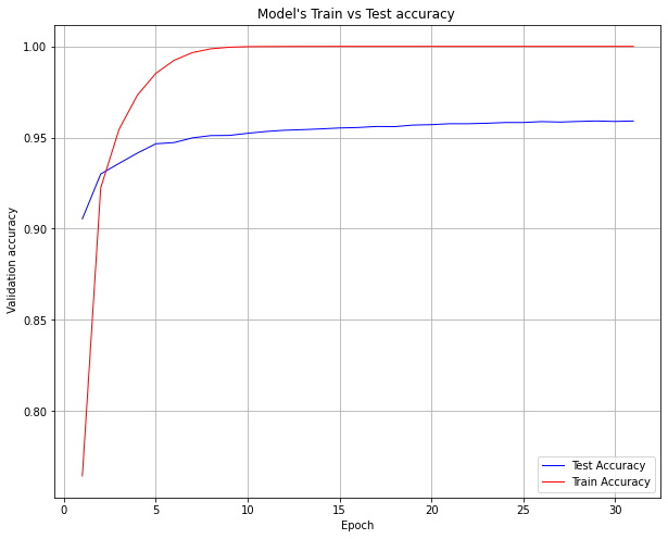
This is to show above early stoping obersvation graphically.

Summary

This notebook provides some starting point to anyone to start coding in tensorflow to build and train models. It also covers some basic tricks like early stopping, tracking metrics etc

Below reference can be checked to find different Optimizers, Loss fuctions, early stopping and other advanced techniques to build upon.

References

https://www.tensorflow.org/

https://keras.io/

https://www.coursera.org/

TensorFlow

Introduction

Import Libraries#

MNIST dataset#

Import MNIST dataset#

Different ways of Building Model

Sequential Model#

Model Architecture#

Create Model#

Model Summary#

Visualize Model#

Compile Model#

Train Model#

Evaluate Model with Test data#

Model built with Functional APIs#

Model Architecture#

Create, Visualize, Train and evaluate the model#

Advanced Model Building Methods#

Custom Layer definition#

Model Architecture#

Create, Visualize, Train and evaluate the model#

Different ways of Training Model

Tracking Training metrics#

Tracking Training & Validation metrics#

Ploting Train vs Test loss#

Early stopping to prevent Overfitting#

Ploting Train vs Test loss#

Summary

References#

Import Libraries

MNIST dataset

Import MNIST dataset

Sequential Model

Model Architecture

Create Model

Model Summary

Visualize Model

Compile Model

Train Model

Evaluate Model with Test data

Model built with Functional APIs

Model Architecture

Create, Visualize, Train and evaluate the model

Advanced Model Building Methods

Custom Layer definition

Model Architecture

Create, Visualize, Train and evaluate the model

Tracking Training metrics

Tracking Training & Validation metrics

Ploting Train vs Test loss

Early stopping to prevent Overfitting

Ploting Train vs Test loss

References